Conference by Gireg Lanoë – machine learning and engine diagnostics

Retranscription de la conférence

Yves Français, PSA

[00:00] Hello everyone. I’m Yves Français, Innovation Project Manager at the PSA Group.

Today, we’re going to talk to you about diagnostic support, and more specifically about the support teams who play an extremely important role. It is the support teams who come to the assistance of dealers or garages when customers, sometimes you, have difficulty identifying the cause of a breakdown. The aim is to make these support teams more efficient and more independent. They have a second extremely important role. They can be in direct contact with suppliers of parts or components, and also with the technical R&D centres, i.e. the specialists and technicians. What we’ve tried to do is make them more independent. In other words, as our colleagues at SNCF said, it is about capitalising on the expertise of the technical teams by creating a toolbox and delivering tools that will enable them to be more independent, so that they don’t need to call on the specialists and experts at the technical centre as much, and can also be more efficient when they work with dealers and garages. This work began three years ago, in a somewhat rudimentary fashion. And a little more concretely, two years ago, with our colleagues at Acsystème. Today, a number of tools are in use with the support teams. I’m going to hand over to Gireg Lanoë from Acsystème to present the topic.

Gireg Lanoë, Acsystème

[01:22] Hello everyone, I’m Gireg Lanoë. I’m a Design Engineer at Acsystème. I’m going to introduce you to the topic starting with a presentation of the problem, the context, the study which was carried out with Matlab Simulink, the tools that we deployed to help PSA and finally the conclusion.

The first part: the context, it’s diagnostics! What is diagnostics? On an engine, there are instructions which are sent by the driver, meaning that he accelerates, brakes and changes gear. Diagnostics: the engine receives messages from the sensors. Diagnostics involve analysing any potential inconsistencies between what has been sent, what the engine is asked to do and what the engine actually does. If there is a discrepancy, depending on the severity of the fault, there will be different types of warning lights that can light up on the dashboard and which will also be visible at the dealership.

The challenge for engine diagnostics is to reduce the number of after-sales service visits, particularly during the warranty period. There is a clear advantage for the manufacturer, because as soon as we can identify the fault, we will be able to repair the correct component and therefore carry out a rapid intervention. Also customer satisfaction: if the customer needs to make several return trips to the garage, satisfaction is likely to drop. Therefore, the challenge is to improve the quality of engine diagnostics, in particular by identifying the source more accurately, so as to reduce intervention time and achieve a good detection compromise. In other words, a detection method will always be a compromise between non-detection and false anomaly. The risk of non-detection is that the day on which the component breaks is not detected: “We’re stopped at the side of the road”. And the false anomaly, on the other hand, will create what is known as the “Christmas tree effect”. In other words, the warning light on the vehicle’s dashboard will come on unexpectedly when in fact there is no fault.

“The exact purpose of a good detection method is to converge on the “Holy Grail”. This is zero false anomalies and zero non-detections, knowing that achieving this would be highly optimistic. ”

Gireg Lanoë, Matlab Expo 2018

[04:15] Diagnostics, as they exist today, are generally based on the observation of a single criterion. That is, it will generally be the observation of a voltage, a control loop deviation, etc. It can be complex to calibrate. Generally, we adjust a threshold on a monovariable, plus an anti-rebound, which means that we wait until the fault is present for a certain number of seconds before validating the fault and reporting it to the customer. So if this threshold is incorrectly calibrated, there is a risk both of non-detection or false anomalies and, with this single criterion analysis, it is difficult to qualify certain types of defect and pinpoint the cause of the customer’s alert. When we took up the issue with PSA, we realised that it was possible to have another diagnostic approach, in particular by using more signals, and by creating models which we called expert models for detection. These expert models are then fine-tuned by a phase portrait analysis, which I’m going to present to you.

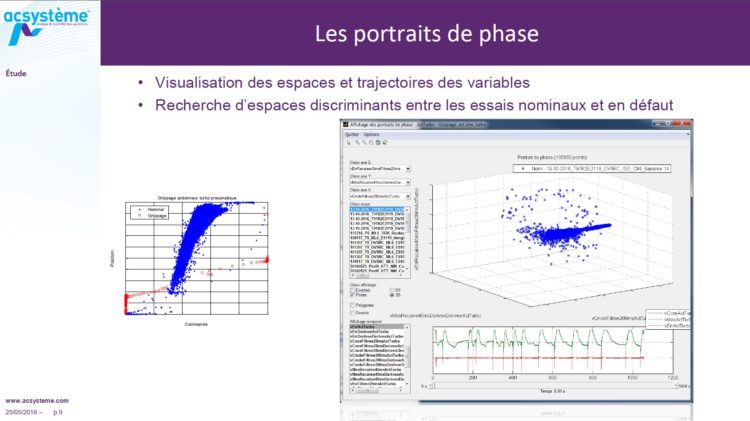
[05:38] What is a phase portrait? Instead of just observing one variable as a function of time, we will observe two variables, one as a function of the other, and see if we can identify a shape visually. This is the purpose of the graph on the left: where we have a scatter plot in blue and a scatter plot in red. The blue scatter plot is the nominal distribution and the red is a faulty test. When we took up the PSA issue, the first objective was to create a tool that, using signals (maximum of 3), could identify three signals which could make it possible to detach a nominal shape and correctly identify a scatter plot in default in the same three-axis representation. The exact purpose of the expert analysis I was talking about earlier would be to create a Simulink that would create boundaries to frame the blue scatter plot, and then, if you go beyond these boundaries, you will find a fault. That was the first approach.

[07:14] The second approach was to switch to a machine learning approach. That is, instead of working by hand, automatically learning the nominal plot and the faulty points. So we set up a machine learning approach, the first stage of which involved creating a database. From tests, identifying the test areas where there was a fault. However, there is expert work to be done beforehand. The second part was learning, with the choice of inputs observed via the phase portrait interface that we saw before, learning using different methods that I will present later, and then threshold calibration, which will enable us to manage the trade-off between false anomalies and non-detection. The third step in the approach is to generate a report and analyse the correct detection/false alarm rates to determine whether or not a detection method is relevant.

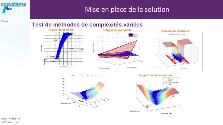
[08:23] The detection methods that were studied were carried out by increasing complexity. Firstly, decision trees were produced, which are a succession of thresholds for reaching a decision, convex bounding polygons, neural networks, Gaussian mixtures and machine vector support, all using Matlab and the Statistic and Neural Networks toolboxes. The little extra touch provided by Acsystème was to adapt to having visualisations which made them a little easier to understand within the limit of two inputs. So this is an illustration of the different methods we were able to test. The first, top left, are decision trees coupled with a principal component analysis to obtain axes that are not parallel to the axes of the two selected inputs, and an analysis using bounding polygons. If you are in the red polygon, it is said that you are not in the blue polygon, so you’re in default. If you are in the blue polygon, you are in nominal.

[09:33] We then tested a neural network approach using a mixture of Gaussian and super vector machines. Here the idea is that you can give a score for each point on the plan. The hypothesis we had was that if it is negative, we are more likely to be on a nominal point, and if it is positive on one point, it is in default. What the tests and validations provided was that we opted for a solution based on neural networks and Gaussian mixtures, because they offer a good compromise between performance and embarcability. Given that the primary criterion is that the number of parameters must be set, for a neural network, a GMM, so that if you generate a Simulink, you don’t need to alter it. We will only modify parameters. We set up an interface that allows thresholds to be calibrated so that, depending on PSA’s choice in this case, it could choose what it wanted in terms of false anomalies and non-detection and select the method that interested it. This can be seen in the graph on the right, where in orange we have the result of a Gaussian mixture method and in blue the neural networks.

The results of these tests showed that it outperformed humans. That means that in some cases we had indicated that the defects were only present in certain areas, and finally we realised that when we repeated the same test the method was telling us: “No, there is a defect here, and there is also a defect here”. Effectively, when we looked at it with an expert eye, we were able to say to ourselves “oh yes, there is indeed a defect that we hadn’t identified previously”.

[11:35] In terms of tool deployment, we have developed two tools for PSA. The first, known as the “expert designer tool”, is used to analyse faults, create new detection models and also score tests. The objective is to carry out the entire machine learning process: annotating, learning and setting the threshold. Then, once the method is satisfactory in the eyes of the expert, store it in a defect database for capitalisation. The aim of this tool is to be used by an expert with a professional eye, who is able to analyse the tests beforehand. The second tool is more of a ‘novice user’ tool that uses the database created by the first tool, and tests that have been carried out on GMP, to create a check-list of faults and suspected faults which could be in the engine that has just been tested. So that is more for use in after-sales service.

[12:43] For this project, we chose the Matlab solution because, given the lack of Matlab licences on all the PCs, we were able to generate tools in .exe format so that they could be used on any workstation. As far as Acsystème is concerned, we have automated the compilation procedure, i.e. we have created a script that selects the right files and automatically generates the “.exe”. The good thing is that we were able to be very responsive with PSA during the debugging phase. As soon as they noticed a problem in the code, they sent us feedback and we were able to deliver a new .exe very quickly. Another advantage is the generation of Simulink models, because the specifications produced at PSA and other manufacturers in general are in Simulink. What is especially practical with neural networks is that the Neural Network Toolbox can be used directly to generate the Simulink which corresponds to the neural network that has been learned. For GMM, we haven’t had the time to do it, but we know it can be coded. What is also interesting is that constraints are taken into account. That means that if PSA has requirements, for example on naming or on the formalism representative of the Simulinks we are able to write code so that the Simulinks generated respect these rules. The only small limitation we had was that on tools compiled in .exe, with the toolboxes available we were not able to use the Simulink model directly. An additional toolbox would therefore be required.

[14:38] Conclusions on the topic. According to the studies we have carried out, the method is fairly generic in the sense that it can be applied to a control loop or a sensor. It provides the after-sales service with details of the origin of faults and, in particular, whether they are electrical or mechanical faults. It can be integrated into an ECU. As I explained earlier, you can export what you’ve learnt in Simulink. We have not gone into this in depth, but we feel that there are opportunities for implementing predictive maintenance. Thank you.